Implementing a simple Artificial Neural Network using Tensorflow
Ever since Tensorflow was released by Google back in Nov-2015, I always wanted to get my hands dirty with it. Being very new to machine learning back then(I still am a noob), the documentation didn’t make much sense to me and having come from Caffe’s background, the way in which a network was described and trained didn’t make any sense either. I recently came across Stephen Welch’s video series Neural Networks Demystified and that inspired me to implement a simple artificial neural network. I choose to implement the same in Tensorflow. (What better way to overcome your fear than to actually face it..eh?)
So here is the problem statement and I’ll walk through the steps of implementing the same.
Problem: Model an OR gate using an ANN
Now, let’s see the truth table for an OR gate
| Input | Output | |
|---|---|---|
| 0 | 0 | 0 |
| 0 | 1 | 1 |
| 1 | 0 | 1 |
| 1 | 1 | 1 |
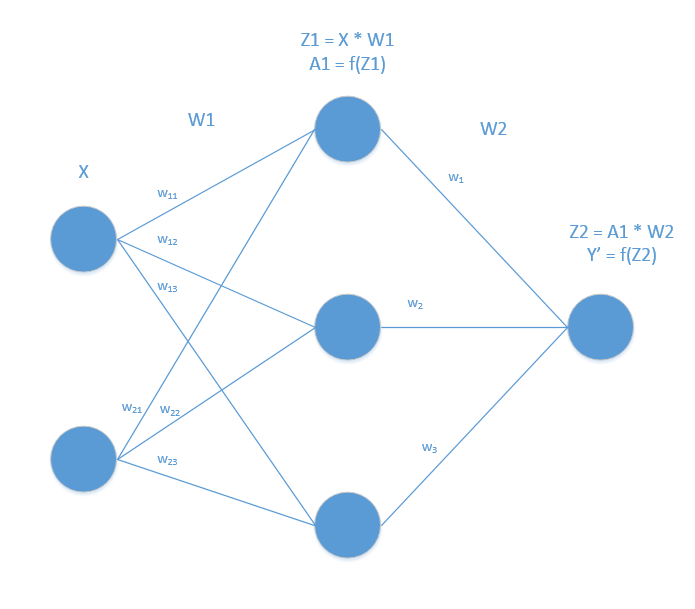
There are two inputs and one output. So our neural network should have two neurons in the input layer and one in the output layer. For simplicity let’s consider only one hidden layer with 3 neurons in it. Our neural network will look something like this:

Let the input be represented by x and output with y. The training data is given below:
x_train = [[0,0], [0,1], [1,0], [1,1]]
y_train = [[0], [1], [1], [1]]
Our weights in first layer is represented in matrix of size 2x3:
W1 = [[w11,w12,w13], [w21,w22,w23]]
Second layer weights again can be represented in a matrix of dimension 3x1
W2 = [[w1, w2, w3]]
The output at first layer z1 is matrix multiplication of input x and weights W1. We will also apply activation function to our output. Activation functions are used to make our model non-linear so that we can fit complex data patterns. This Quora thread has nice explanation of activation functions. We will choose tanh or the hyberbolic tangent function as our activation function. It is represented as follows:

So, the first layer ouput can be written as:
A1 = f(z1), where z1 = matmul(x, W1)
similarly, output of final layer y' = f(z2) where z2 = matmul(A1, W2)
We have represented out output as y' since it is the predicted output from the system and not the actual output.
We should then define our cost function which is a measure of how bad or good our system is. Our aim is to minimize the cost. We will choose our cost function as sum of the squared error for each training data. We will minimize the cost using the Gradient Descent method.
Once we have outlined our network and other considerations, it’s time for us to implement the same in Tensorflow.
import tensorflow as tf

x = tf.placeholder(tf.float32, [None, 2])
y = tf.placeholder(tf.float32)

W1 = tf.Variable(tf.random_normal([2,3]))
W2 = tf.Variable(tf.random_normal([3,1]))

Z1 = tf.matmul(x, W1)
A1 = tf.tanh(Z1)

Z2 = tf.matmul(A1, W2)
y_ = tf.tanh(Z2)

cost = 0.5 * tf.reduce_sum(tf.square(y_ - y), 1)

optimizer = tf.train.GradientDescentOptimizer(0.1)
train = optimizer.minimize(cost)

x_train = [[0, 0], [0, 1], [1, 0], [1, 1]]
y_train = [[0], [1], [1], [1]]

sess = tf.Session()
init = tf.global_variables_initializer()
sess.run(init)

print(sess.run(y_, {x:x_train}))
for i in range(10000):
    sess.run(train, {x:x_train, y:y_train})

print(sess.run(y_, {x:x_train}))